El Blog de @Aethilas: Using Excel for SEO – the Grand Collection of Tips

Using Excel for SEO – the Grand Collection of Tips: "

You probably know that I am a big Excel fanatic (though not an expert). To me, Excel has always been the ultimate SEO and productivity tool.

I’ve been collecting Excel tutorials for years and this post lists the most useful (yet, the least geeky) of them: no matter which SEO task you have come across, chances are you’ll find one of the following tutorials handy:

1. Export Any Data to Excel

Any well-known keyword research or traffic analytics tool has the “Export-to-CSV” feature and a CSV file is easy to open in Excel – so converting your data into Excel shouldn’t be a problem.

If you still you need some examples, I did a post quite some time ago listing many ways to export your backlink data to Excel; for instance:

With Yahoo! SiteExplorer you can export results to TSV file and open it as Excel;

With Google Analytics you can save the report of referring domains (enhanced with plenty of browsing data per each linking domain: bounce rate, time spent on site; pages per visit, etc).

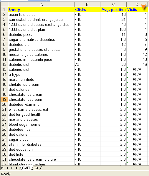
You can export any search results that provide RSS feed to Google Spreadsheets using =ImportFeed(“feed URL”) formula and then save as Excel:

Export Excel

2. Excel for Keyword Research: a Pivot Table and a (Conditional) Formatting

1. Create a Pivot Table to easily Re-Arrange the Keywords

This post by Richard Baxter on creating a pivot table and a beautiful chart using Excel offers a step-by-step tutorial on how to re-organize your data to run various types of analysis. In short, the steps are as follows:

Collect your data and create a Master table (more often than not, so to create your master table, you just need to export the required range of data from the tool you are using and open the file using Excel).
- If you are using several tools, you may want to combine the data in one table – this post on using VLOOKUP query will save your life!

Create a Pivot Table on a new sheet: “Insert > PivotTable > PivotChart“ and choose your table to serve the basis of the Pivot table;

Add axis fields, values, column labels and filters: The PivotTable Field List uses drag and drop functionality to enable you to populate those little white squares with values. As you add values, the table on the left begins to form.

Pivot Table

A pivot table feature allows for plenty of data manipulation options that consequently offers a wide range of research types. Here’s another post giving a detailed tutorial on creating a pivot table and using it for keyword research – so if you still have any questions, refer to it to make things even clearer.

2. Use “Find and Replace” Feature to Visualize the Keyword Patterns

While a pivot table lets you re-arrange the data and create cool charts, conditional formatting allows you to visualize the data sets using different colors. I did a post once on finding your most frequent modifiers using Excel, and here are the steps:

Use CTRL+F (“Find and Replace” feature);

Click “Find and Replace” tab;

Type the word you think may be frequently used with your core term,

Click “Options” button;

Choose to “replace with” format;

Click “Patterns” tab;

Choose the color you want to highlight the cell containing the word:

Click OK and then “Replace All”;

You should then see how many times the word was used, plus the cells containing it will be highlighted.

Conditional formatting

Conditional formatting works the similar way but it can be used to highlight the cells while you are creating the spreadsheet. For example, if you are using Excel to create and track your meta tags, conditional formatting can visualize meta tag character count. Simply use Red/Yellow/Green for good length and warning zones. This keeps you in a quick reference just out of the peripheral.

3. Use =VLOOKUP to compare and combine data exported from different sources:

This post on comparing Google Webmaster Tools Data with Google Analytics Data provides a detailed tutorial on how you can merge any type of statistics data: Keyword Rankings and Keyword Volume, Google Rankings data and Traffic data, Backlinks and Traffic Sources, etc:

Excel merge

3. Excel for Link Building: URL Manipulations

I use Excel for link building process tracking as well as for reporting. The basic “sorting” Excel feature (known by everyone, I guess) makes it much easier to re-arrange the data to find links on the same topic, with the same Google PR, etc.

This section looks at a bit more complex hacks: Excel formulas and tutorials for the URL manipulation.

1. Extract All URLs from the List of Linked Words

It happens very often that you have a list of linked words in Excel and you need to see the full address of each link. Extracting each address one by one is tedious. To automate the task, you will need to create a quick macro – don’t worry, here’s an instruction allowing even a very basic newbie to create one:

Open Visual Basic Editor (use ALT + F11 shortcut);

Navigate Insert -> Module to adds a module

Paste the code below

Close the Visual Basic Editor (use ALT + Q)

Sub ExtractHL()

Dim HL As Hyperlink

For Each HL In ActiveSheet.Hyperlinks

HL.Range.Offset(0, 1).Value = HL.Address

Next

End Sub

Now use the macro:

Navigate Tools -> Macro -> Macros (or use ALT + F8 shortcut);

Make sure “Extract HL” is chosen and click Run

You are done! The macro will find each hyperlink in a worksheet, extract each one’s URL, and stick that URL in the cell directly to the right of the hyperlink.

Extract URLs

2. Make the List of URLs Active

Another common case is: you export tons of data and end up with hundreds of unlinked URLs. You could go double-clicking on each to activate one by one but this will take too much time. Here’s a quick tutorial on how you can do that:

Repeat steps 1 to 4 from the above tip but use this code: